42 modify legend labels excel 2013
Learn Excel 2013 - "Chart Legend Changes": Podcast #1693 Referring to Podcast #1408 where Bill showed us how to moved a Chart Legend, Bill begins today's podcast by describing and demonstrating not only the Moving ... Sort legend items in Excel charts - teylyn Finally, go back to the data for the helper series up in I2 to I5 and change the values for the helper series to zeros. Now your chart should look like this: step 6. Result: The series order is yellow, blue, pink, green, but the legend items are sorted alphabetically, i.e. apples - pink. bananas - green.
Move and Align Chart Titles, Labels, Legends with the ... - Excel Campus Select the element in the chart you want to move (title, data labels, legend, plot area). On the add-in window press the "Move Selected Object with Arrow Keys" button. This is a toggle button and you want to press it down to turn on the arrow keys. Press any of the arrow keys on the keyboard to move the chart element.

Modify legend labels excel 2013
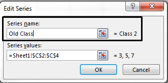
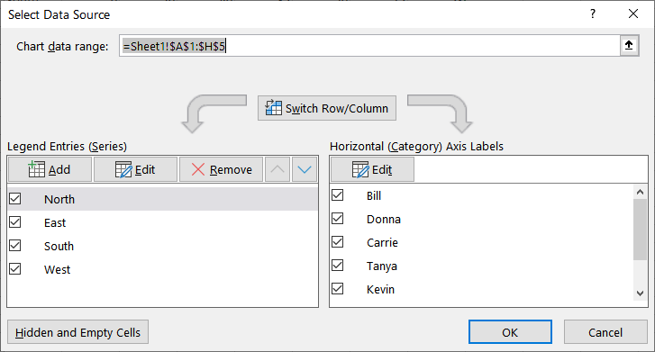
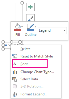
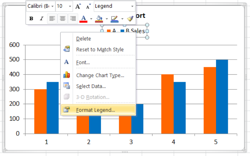
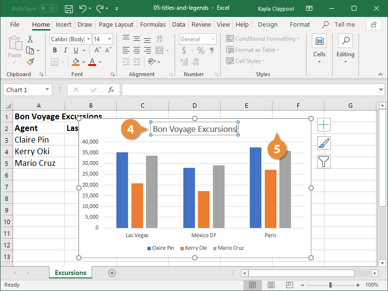
How to Edit Legend in Excel | Excelchat Change legend name Change Series Name in Select Data Step 1. Right-click anywhere on the chart and click Select Data Figure 4. Change legend text through Select Data Step 2. Select the series Brand A and click Edit Figure 5. Edit Series in Excel The Edit Series dialog box will pop-up. Figure 6. Edit Series preview pane Step 3. Legends in Excel Charts - Formats, Size, Shape, and Position When you change the font to a legible size, like 8 pt, the legend moves to near the right position and the chart itself expands to its original size. The default placements, at least right and top, are okay. But Excel leaves too much space around the legend and between the legend and the rest of the chart. Change legend names - support.microsoft.com Select your chart in Excel, and click Design > Select Data. Click on the legend name you want to change in the Select Data Source dialog box, and click Edit. Note: You can update Legend Entries and Axis Label names from this view, and multiple Edit options might be available. Type a legend name into the Series name text box, and click OK.
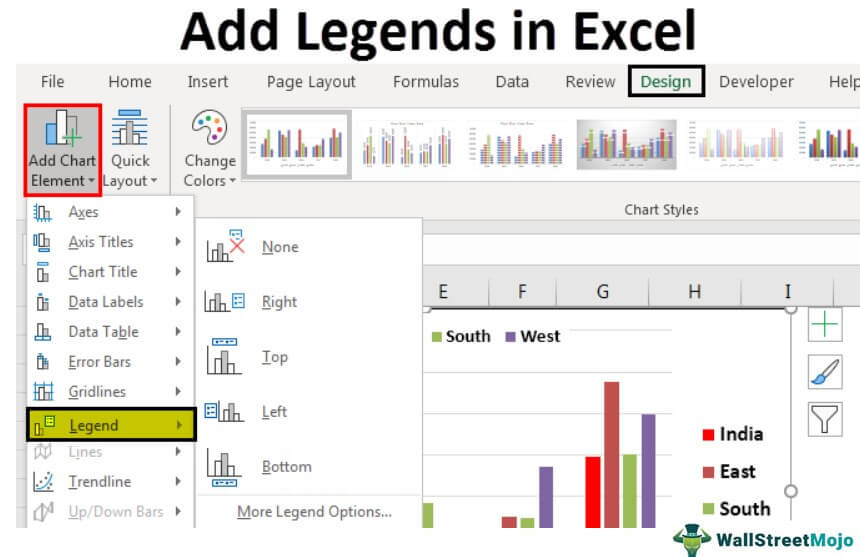
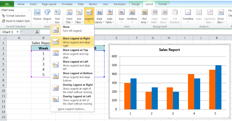
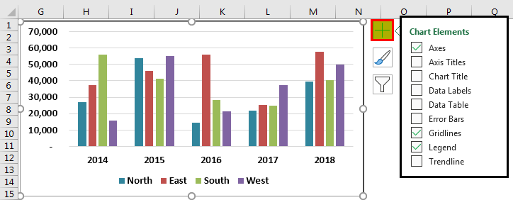
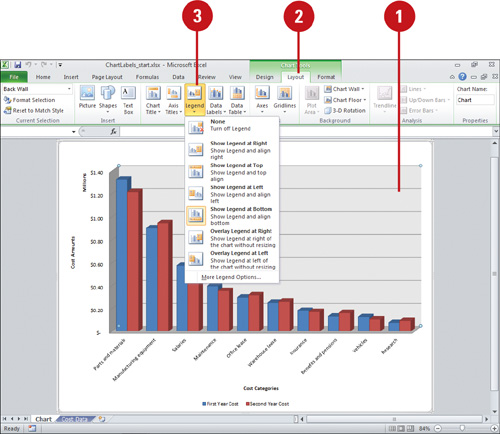
Modify legend labels excel 2013. How to Print Labels from Excel - Lifewire Select Mailings > Write & Insert Fields > Update Labels . Once you have the Excel spreadsheet and the Word document set up, you can merge the information and print your labels. Click Finish & Merge in the Finish group on the Mailings tab. Click Edit Individual Documents to preview how your printed labels will appear. Select All > OK . Legends in Excel | How to Add legends in Excel Chart? - WallStreetMojo For changing the positioning of the legends in Excel 2013 and later versions, there is a small PLUS button on the right-hand side of the chart. If we click on that PLUS icon, we will see all the chart elements. Here we can change, enable, and disable all the chart elements. How to make a histogram in Excel 2019, 2016, 2013 and 2010 - Ablebits.com To add the Data Analysis add-in to your Excel, perform the following steps: In Excel 2010, Excel 2013, Excel 2016, and Excel 2019, click File > Options. In Excel 2007, click the Microsoft Office button, and then click Excel Options. In the Excel Options dialog, click Add-Ins on the left sidebar, select Excel Add-ins in the Manage box, and click ... Modify chart legend entries - support.microsoft.com Edit legend entries in the Select Data Source dialog box Edit legend entries on the worksheet On the worksheet, click the cell that contains the name of the data series that appears as an entry in the chart legend. Type the new name, and then press ENTER. The new name automatically appears in the legend on the chart.
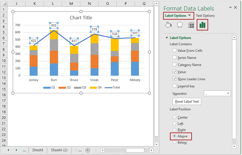
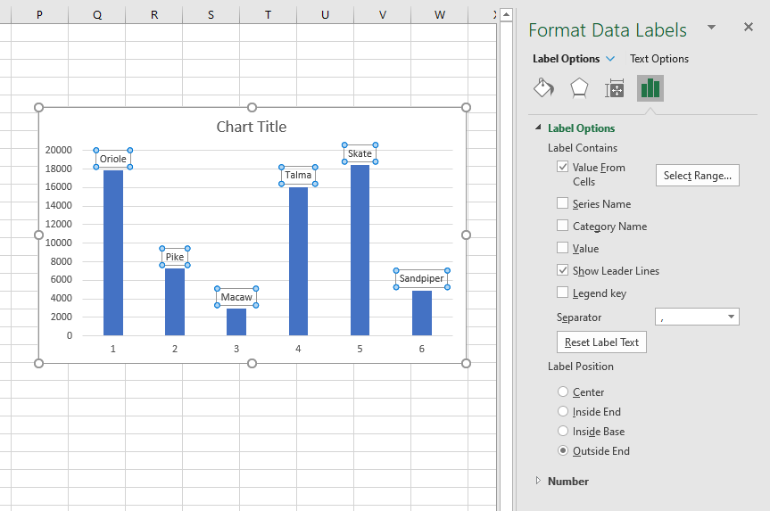
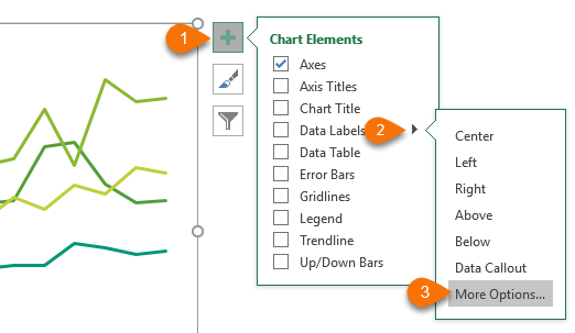
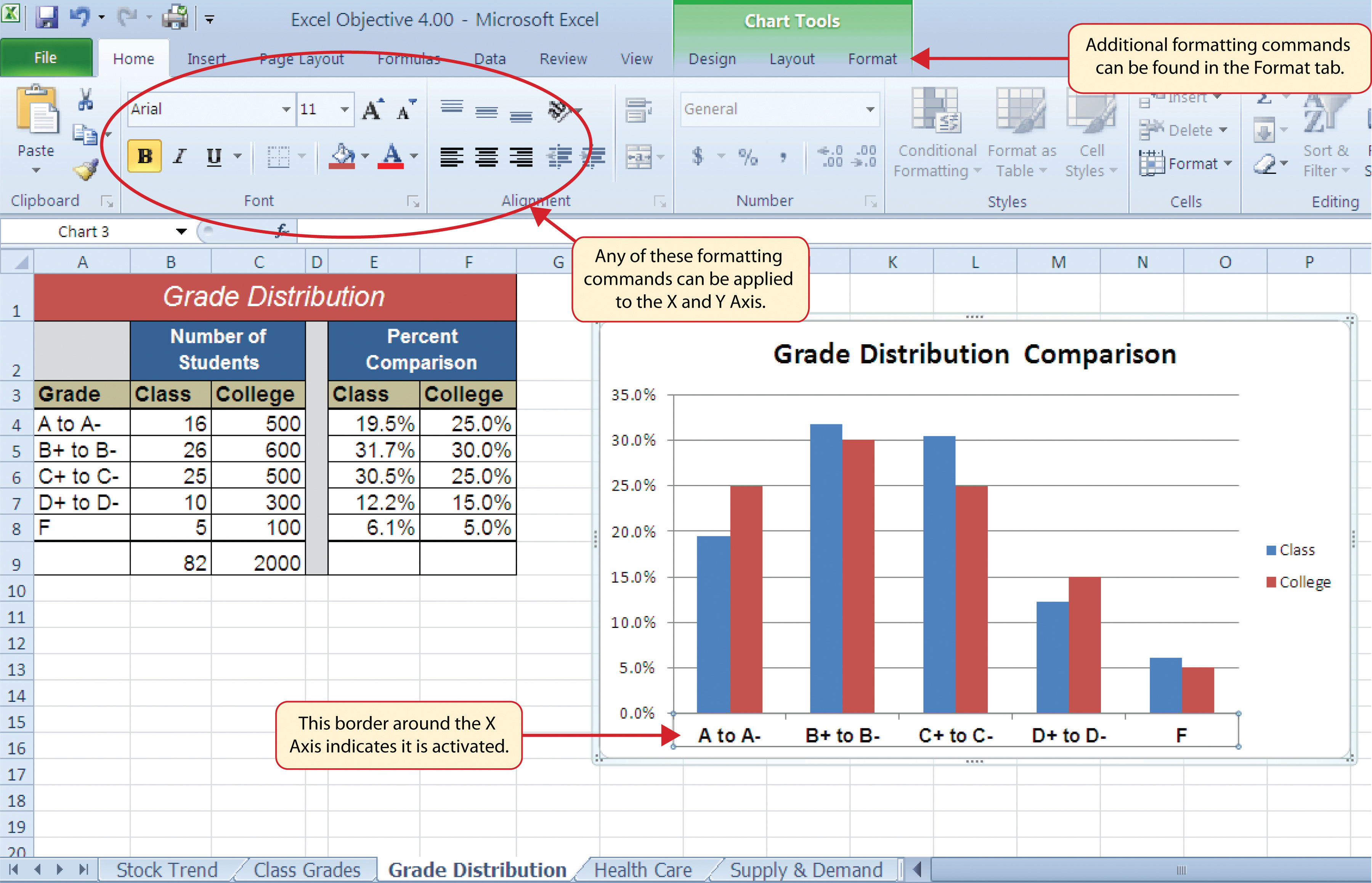
Excel charts: add title, customize chart axis, legend and data labels To change what is displayed on the data labels in your chart, click the Chart Elements button > Data Labels > More options… This will bring up the Format Data Labels pane on the right of your worksheet. Switch to the Label Options tab, and select the option (s) you want under Label Contains: How to change default chart legend text from "Total?" Answers. I'm afraid you can't change the label of the legend in pivot chart. As a workaround, we can add a calculated filed in pivot table ,set the value of this filed as 0. Then in pivot chart ,choose 'no line' in 'Line' dropdown list. For adding the Power Trendline, right click the Actual line->add Trendline->choose Power. How to Edit Legend Entries in Excel: 9 Steps (with Pictures) - wikiHow Select a legend entry in the "Legend entries (Series)" box. This box lists all the legend entries in your chart. Find the entry you want to edit here, and click on it to select it. 6 Click the Edit button. This will allow you to edit the selected entry's name and data values. On some versions of Excel, you won't see an Edit button. Dynamically Label Excel Chart Series Lines - My Online Training Hub Step 1: Duplicate the Series. The first trick here is that we have 2 series for each region; one for the line and one for the label, as you can see in the table below: Select columns B:J and insert a line chart (do not include column A). To modify the axis so the Year and Month labels are nested; right-click the chart > Select Data > Edit the ...
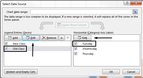
Format and customize Excel 2013 charts quickly with the new Formatting ... The new Excel makes creating and customizing charts simpler and more intuitive. One part of the fluid new experience is the Formatting Task pane, which replaces the Format dialog box. The new Formatting Task pane is the single source for formatting--all of the different styling options are consolidated in one place. With this single task pane, you can modify not only charts, but also shapes ... Adding rich data labels to charts in Excel 2013 | Microsoft 365 Blog You can do this by adjusting the zoom control on the bottom right corner of Excel's chrome. Then, select the value in the data label and hit the right-arrow key on your keyboard. The story behind the data in our example is that the temperature increased significantly on Wednesday and that appeared to help drive up business at the lemonade stand. Adjusting the Angle of Axis Labels (Microsoft Excel) - ExcelTips (ribbon) Right-click the axis labels whose angle you want to adjust. Excel displays a Context menu. Click the Format Axis option. Excel displays the Format Axis task pane at the right side of the screen. Click the Text Options link in the task pane. Excel changes the tools that appear just below the link. Click the Textbox tool. How to change legend in Excel chart - Excel Tutorials - OfficeTuts Excel Click Edit under Legend Entries (Series). Inside the Edit Series window, in the Series name, there is a reference to the name of the table. Change this entry to Joe's earnings and click OK. Now, click Edit under Horizontal (Category) Axis Labels . Insert a list of names into the Series name box. = {"Mon","Tue","Wed","Thu","Fri","Sat"} Click OK.
Change axis labels in a chart
How to Add Axis Labels in Excel 2013 - YouTube This is a tutorial on how to add axis labels in Excel 2013. Axis labels, for the most part, are added immediately to your chart once it is created. in Excel 2013, when the chart is highlighted, you...

Creating Graphs in Excel 2013
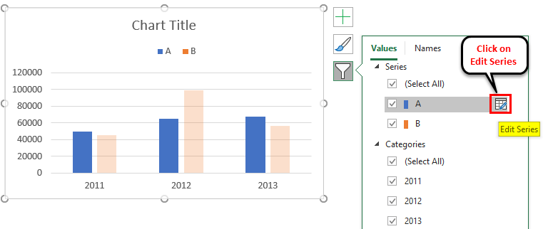
Excel Chart Legend | How to Add and Format Chart Legend? - WallStreetMojo First, we need to go to the option "Chart Filters.". It helps to edit and modify the names and areas of the chart elements. Then click on "Select Data," as highlighted below in red. When we select the above option, a pop-up menu called the "Select Data Source" screen appears. In addition, there is an option of "Edit.".
Add and format a chart legend
Excel 2013 legend entries in wrong order on stacked column charts Right-click on the legend and choose FORMAT LEGEND. In Excel 2013, change the LEGEND POSITION to LEFT or RIGHT. You may want to re-size the Legend Box again, but you'll find the entries in the right order. I've forgotten what the FORMAT LEGEND dialogue box looks like in earlier versions of Excel, but you just basically follow the same steps.
Change legend names
How to Customize Chart Elements in Excel 2013 - dummies To add data labels to your selected chart and position them, click the Chart Elements button next to the chart and then select the Data Labels check box before you select one of the following options on its continuation menu: Center to position the data labels in the middle of each data point
How to change legend text in Microsoft excel
How to change the order of your chart legend - Excel Tips & Tricks ... Under the Data section, click Select Data. Step 2: In the Select Data Source pop up, under the Legend Entries section, select the item to be reallocated and, using the up or down arrow on the top right, reposition the items in the desired order.
How to add total labels to stacked column chart in Excel?
Changing Axis Labels in PowerPoint 2013 for Windows - Indezine Now, let us learn how to change category axis labels. First select your chart. Then, click the Edit Data button as shown highlighted in red within Figure 7 ,below, within the Charts Tools Design tab of the Ribbon. This opens an instance of Excel with your chart data. Notice the category names shown highlighted in blue. Figure 7: Edit Data button

Excel charts: add title, customize chart axis, legend and ...
The Select Data Source Dialog Box in Excel 2013 - dummies In Excel 2013, when you click the Select Data command button on the Design tab of the Chart Tools contextual tab (or press Alt+JCE), Excel opens a Select Data S ... Edit the labels used to identify the data series in the legend or on the horizontal (category) by clicking the Edit button on the Legend Entries (Series) or Horizontal (Categories ...
Legends in Excel | How to Add legends in Excel Chart?
Order of Legend Entries in Excel Charts - Peltier Tech In a bar chart, whether clustered or stacked, entries in a vertically aligned legend are listed in the same order as they appear in the chart. The alignment matches the order of the bars in the chart, even if the order of the bars is reversed by plotting an axis in the reverse order. Effect of Stacking, Axis, and Chart Type on Legend Entry Order
Microsoft Office Excel 2013 Tutorial: Adding Chart Titles and Legends | K Alliance
How to modify Chart legends in Excel 2013 - Stack Overflow Apr 14, 2014 at 16:22. Right-click any column in the chart and select "Select Data" in the context menu. In the next dialog, select one of the series and click the Edit button. - teylyn.

Move and Align Chart Titles, Labels, Legends with the Arrow ...
Change legend names - support.microsoft.com Select your chart in Excel, and click Design > Select Data. Click on the legend name you want to change in the Select Data Source dialog box, and click Edit. Note: You can update Legend Entries and Axis Label names from this view, and multiple Edit options might be available. Type a legend name into the Series name text box, and click OK.
How to Edit Legend in Excel | Excelchat
Legends in Excel Charts - Formats, Size, Shape, and Position When you change the font to a legible size, like 8 pt, the legend moves to near the right position and the chart itself expands to its original size. The default placements, at least right and top, are okay. But Excel leaves too much space around the legend and between the legend and the rest of the chart.

Directly Labeling in Excel
How to Edit Legend in Excel | Excelchat Change legend name Change Series Name in Select Data Step 1. Right-click anywhere on the chart and click Select Data Figure 4. Change legend text through Select Data Step 2. Select the series Brand A and click Edit Figure 5. Edit Series in Excel The Edit Series dialog box will pop-up. Figure 6. Edit Series preview pane Step 3.
Analyzing Data with Tables and Charts in Microsoft Excel 2013 ...

Change axis labels in a chart in Office
Analyzing Data with Tables and Charts in Microsoft Excel 2013 ...
Custom data labels in a chart
Change legend names
Excel Charts with Dynamic Title and Legend Labels (with Steps)
Dynamically Label Excel Chart Series Lines • My Online ...
How-to Make a WSJ Excel Pie Chart with Labels Both Inside and ...
Adjusting the Order of Items in a Chart Legend (Microsoft Excel)
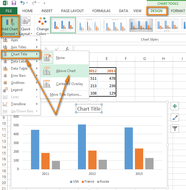
How to add titles to Excel charts in a minute.

Legends in Excel | How to Add legends in Excel Chart?

How to change the order of your chart legend - Excel Tips ...
Add and format a chart legend

264. How can I make an Excel chart refer to column or row ...
How to Edit Legend in Excel | Excelchat
Legends in Excel | How to Add legends in Excel Chart?
How to show, hide, and edit Legend in Excel
Microsoft Excel 2010 : Creating and Modifying Charts ...
Legend Entry Tricks in Excel Charts - Peltier Tech

Excel: Clustered Column Chart with Percent of Month ...
Add a legend, gridlines, and other markings in Numbers on Mac ...
How to Edit a Legend in Excel | CustomGuide
/simplexct/BlogPic-3a631.png)
How to Directly Label Stacked Column Charts in Excel

Microsoft Excel Tutorials: The Chart Layout Panels
Formatting Charts
10 Tips To Make Your Excel Charts Sexier

Excel Custom Chart Labels • My Online Training Hub

How to fix wrapped data labels in a pie chart | Sage Intelligence
Change legend names

How to Make an Excel Pie Chart
Post a Comment for "42 modify legend labels excel 2013"