43 excel donut chart labels

How to Create Doughnut Chart in Excel? - EDUCBA Now we will create a doughnut chart as similar to the previous single doughnut chart. Select the data alone without headers, as shown in the below image. Click on the Insert menu. Go to charts select the PIE chart drop-down menu. From Dropdown, select the doughnut symbol. Then the below chart will appear on the screen with two doughnut rings. How to create a creative multi-layer Doughnut Chart in Excel By default, all doughnut chart layers have a borderline. As this border line is only disrupting the look, you should remove it for all borders first. After that, select the outer layer of the second (also second biggest) data point and set the fill to No fill. For the third data point we apply the same technique to the two outer layers, and so on.

How to create doughnut chart in Excel? - extendoffice.com In Excel 2013, click Insert > Insert Pie or Doughnut Chart > Doughnut. See screenshot: 2. Then a doughnut chart is inserted in your worksheet. Now you can right click at all series and select Add Data Labels from the context menu to add the data labels. See screenshots: Now a simple doughnut chart is created.

Excel donut chart labels

donut chart labels - Microsoft Community Sep 26, 2013 · Click the chart. On the Format tab, in the Size group, enter the size that you want in the Shape Height and Shape Width box. Tip For our doughnut chart, we set the shape height to 4" and the shape width to 5.5". To change the size of the doughnut hole, do the following: How to Create Doughnut Excel Chart? - WallStreetMojo doughnut chart is a type of chart in excel whose function of visualization is just similar to pie charts, the categories represented in this chart are parts and together they represent the whole data in the chart, only the data which are in rows or columns only can be used in creating a doughnut chart in excel, however it is advised to use this … Progress Doughnut Chart with Conditional Formatting in Excel The entire chart will be shaded with the progress complete color, and we can display the progress percentage in the label to show that it is greater than 100%. Step 2 - Insert the Doughnut Chart With the data range set up, we can now insert the doughnut chart from the Insert tab on the Ribbon. The Doughnut Chart is in the Pie Chart drop-down menu.

Excel donut chart labels. Interactive Donut Chart - Beat Excel! Now select and copy the first gray area in Sheet 2 that includes blue donut part and paste it as a linked picture to cell B2 of Sheet 1. Click on this picture and type =Chart inside the formula bar. Do the same with the label but this time place it in the middle of the gray area in Sheet 1. While on Sheet 1, insert a donut chart as shown below. Labels for pie and doughnut charts - Support Center To format labels for pie and doughnut charts: 1. Select your chart or a single slice. Turn the slider on to Show Label. 2. Use the sliders to choose whether to include Name, Value, and Percent. 3. Use the Precision setting allows you to determine how many digits display for numeric values. 4. How to make doughnut chart with outside end labels? - Simple Excel VBA ... In the doughnut type charts Excel gives You no option to change the position of data label. The only setting is to have them inside the chart. Excel Doughnut chart with leader lines - teylyn Step 1 - doughnut chart with data labels Step 2 -Add the same data series as a pie chart Next, select the data again, categories and values. Copy the data, then click the chart and use the Paste Special command. Specify that the data is a new series and hit OK. You will see the new data series as an outer ring on the doughnut chart.

How to Create a Double Doughnut Chart in Excel - Statology Step 3: Add a layer to create a double doughnut chart. Right click on the doughnut chart and click Select Data. In the new window that pops up, click Add to add a new data series. For Series values, type in the range of values fpr Quarter 2 revenue: Click OK. Excel Charts - Doughnut Chart - Tutorialspoint Step 2 − Select the data. Step 3 − On the INSERT tab, in the Charts group, click the Pie chart icon on the Ribbon. It is used to insert a Doughnut chart also. You will see the different types of Doughnut charts available. Step 4 − Point your mouse on the Doughnut icon. A preview of that chart type will be shown on the worksheet. Excel 2007 Doughnut chart Label Bug When I generate a doughnut chart with two series of data and activate displaying the category names for the datatpoints, then for the 2nd series Excel 2007 displays the names from the 1st series! E.g. Series 1 with A, B and C, Series 2 with A1, A2, B1, B2, B3, C1 and C2. Either the Series 1 gets the labels A1, A2, B1 from series 2. Present your data in a doughnut chart - support.microsoft.com To add text labels with arrows that point to the doughnut rings, do the following: On the Layout tab, in the Insert group, click Text Box. Click on the chart where you want to place the text box, type the text that you want, and then press ENTER.

Add / Move Data Labels in Charts - Excel & Google Sheets Add and Move Data Labels in Google Sheets. Double Click Chart. Select Customize under Chart Editor. Select Series. 4. Check Data Labels. 5. Select which Position to move the data labels in comparison to the bars. Fix label position in doughnut chart? | MrExcel Message Board Turn off data labels. Insert a Text box in to the middle of the donut, select the edge of the text box and in the formula bar hit = then select the cell that contains the progress figure. You can format this to however you want it, it will update and it won't move. Click to expand... Oh wow! I always thought text-boxes were just text-boxes. How to Make a Doughnut Chart in Excel | EdrawMax Online Step 1: Select Chart Type. When you open a new drawing page in EdrawMax, go to Insert tab, click Chart or press Ctrl + Alt + R directly to open the Insert Chart window so that you can choose the desired chart type. Here we need to insert a basic doughnut chart into the drawing page, so we can just select " Doughnut Chart " on the window and ... excel - Positioning labels on a donut-chart - Stack Overflow Show activity on this post. I have the following code which attempts to add a datalabel to a point in a combined donut/pie-chart: For Each co In .ChartObjects With co.Chart.FullSeriesCollection ("Grøn pil").Points (2) .HasDataLabel = True With .DataLabel .Position = xlLabelPositionOutsideEnd .Format.AutoShapeType = msoShapeRectangle .Format ...

Hierarchical Series (CTP) - Doughnut Chart - WPF

How to add leader lines to doughnut chart in Excel? Select data and click Insert > Other Charts > Doughnut. In Excel 2013, click Insert > Insert Pie or Doughnut Chart > Doughnut. 2. Select your original data again, and copy it by pressing Ctrl + C simultaneously, and then click at the inserted doughnut chart, then go to click Home > Paste > Paste Special. See screenshot: 3.

5 New Charts to Visually Display Data in Excel 2019 - dummies

Excel Doughnut Chart in 3 minutes - Watch Free Excel Video ... - YouTube Doughnut charts is cirular graph which display data in rings, where each ring represents a data series. In Doughnut Chart percentages are displayed in data l...

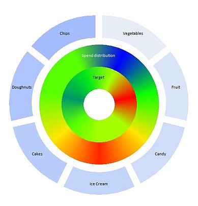
Wow! Heat Map Donut Chart! - Peltier Tech Blog

Change the format of data labels in a chart To get there, after adding your data labels, select the data label to format, and then click Chart Elements > Data Labels > More Options. To go to the appropriate area, click one of the four icons ( Fill & Line, Effects, Size & Properties ( Layout & Properties in Outlook or Word), or Label Options) shown here.

30 Tableau Pie Chart Percentage Label - Label Design Ideas 2020

Question: labels in an Excel doughnut chart - Microsoft Tech Community Nov 15, 2020 · Open your Excel document and click on your chart. In the upper bar you will find the "Diagram Tools". Click on the "Design" tab. In the "Data" group, click the "Select data" button. In the right window you will find the "Horizontal axis label". Click on "Edit". Now enter your desired names or values for the legend.

Donut Chart - Learn about this chart and tools to create it

Leader lines for Excel doughnut charts - Site Title Step 1 - create the doughnut chart. First, let's create a doughnut chart straight from the standards, delete the legend, change the wedge colors and add data labels for category and value. That will look something like this: Step 1 - doughnut chart with data labels.

Half Donut Chart (Infographic Style ) - Beat Excel!

Curve Text in Doughnut chart - Excel Help Forum Re: Curve Text in Doughnut chart. You can link WordArt to a cell using a formula. Just select the shape, click into the formula bar, type = and then select the cell and press Enter. Please remember to mark your thread 'Solved' when appropriate.

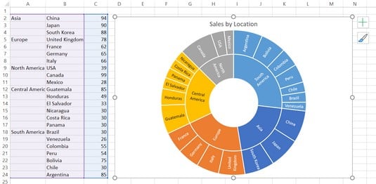
Nested donut chart (also known as Multi-level doughnut chart, Multi-series doughnut chart ...

Doughnut Chart in Excel - GeeksforGeeks Follow the below steps to insert a doughnut chart with single data series: Insert the data in the spreadsheet. We will take the example of data showing the sales of apple between January - August. Select the data (A2:A9, B2:B9). Click on Insert Tab. Select your desired Doughnut chart (Doughnut, Exploded doughnut), under the Other charts.

chart.js - Aligning of doughnut charts to top in chartjs - Stack Overflow

Progress Doughnut Chart with Conditional Formatting in Excel The entire chart will be shaded with the progress complete color, and we can display the progress percentage in the label to show that it is greater than 100%. Step 2 - Insert the Doughnut Chart With the data range set up, we can now insert the doughnut chart from the Insert tab on the Ribbon. The Doughnut Chart is in the Pie Chart drop-down menu.

Share :