40 how to add data labels to a pie chart in excel on mac

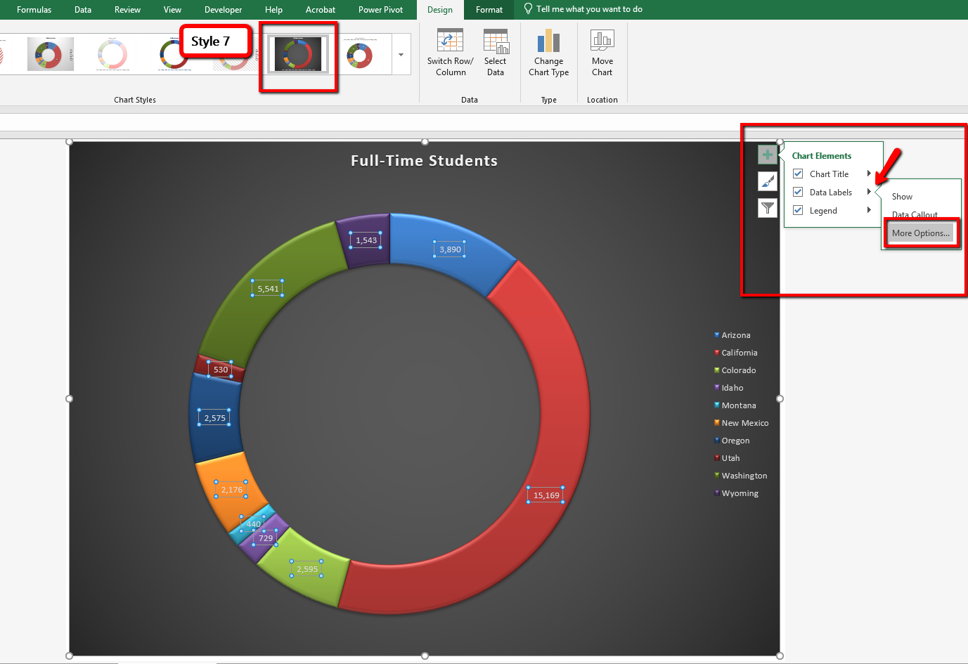
How to make pie charts in excel - javatpoint How to make pie charts in excel with topics of ribbon and tabs, quick access toolbar, mini toolbar, buttons, worksheet, data manipulation, function, formula, vlookup, isna and more. ... Worksheet, Row, Column Moving on Worksheet Enter Data Select Data Delete Data Move Data Copy Paste Data Spell Check Insert Symbols. Excel Calculation. Addition ... Add or remove data labels in a chart - support.microsoft.com Click the data series or chart. To label one data point, after clicking the series, click that data point. In the upper right corner, next to the chart, click Add Chart Element > Data Labels. To change the location, click the arrow, and choose an option. If you want to show your data label inside a text bubble shape, click Data Callout.

How to Create a Pie Chart in Excel | Smartsheet If want the category names to appear on or near the chart, right-click on the chart and click Add Data Labels …. By default, the numerical values are added. To add other labels, such as the categorical values or the percentage of the total that each category represents, right-click on the chart, then click Format Data Labels ….

How to add data labels to a pie chart in excel on mac

How to Make a Pie Chart in Excel — Everything You Need to Know Changing the Position of your Pie Chart. 1. To change position of data labels, click Chart Tools > Layout > Data Labels. 2. Set the desired data label from drop-down options (outside end shown here). Formatting Slices. 1. Slices can also be formatted under Chart Tools > Format. To format slices, select Shape Effects. Microsoft Excel Tutorials: Add Data Labels to a Pie Chart To add the numbers from our E column (the viewing figures), left click on the pie chart itself to select it: The chart is selected when you can see all those blue circles surrounding it. Now right click the chart. You should get the following menu: From the menu, select Add Data Labels. New data labels will then appear on your chart: How to create Custom Data Labels in Excel Charts Add data labels Create a simple line chart while selecting the first two columns only. Now Add Regular Data Labels. Two ways to do it. Click on the Plus sign next to the chart and choose the Data Labels option. We do NOT want the data to be shown. To customize it, click on the arrow next to Data Labels and choose More Options …

How to add data labels to a pie chart in excel on mac. Add a Data Callout Label to Charts in Excel 2013 In the upper right corner, next to your chart, click the Chart Elements button (plus sign), and then click Data Labels. A right pointing arrow will appear, click on this arrow to view the submenu. Select Data Callout. Once the Data Callout Labels have been added, you can re-position them by clicking on their borders and dragging to a new position. How to Create and Format a Pie Chart in Excel - Lifewire To add data labels to a pie chart: Select the plot area of the pie chart. Right-click the chart. Select Add Data Labels . Select Add Data Labels. In this example, the sales for each cookie is added to the slices of the pie chart. Change Colors Excel charts: add title, customize chart axis, legend and data labels ... To add a label to one data point, click that data point after selecting the series. Click the Chart Elements button, and select the Data Labels option. For example, this is how we can add labels to one of the data series in our Excel chart: For specific chart types, such as pie chart, you can also choose the labels location. How to format the data labels in Excel:Mac 2011 when showing a ... Try clicking on Column or Row you want to set. Go to Format Menu Click cells Click on Currency Change number of places to 0 (zero) (if in accounting do the same thing. _________ Disclaimer: The questions, discussions, opinions, replies & answers I create, are solely mine and mine alone, and do not reflect upon my position as a Community Moderator.

Pie Chart in Excel | How to Create Pie Chart - EDUCBA Step 1: Select the data to go to Insert, click on PIE, and select 3-D pie chart. Step 2: Now, it instantly creates the 3-D pie chart for you. Step 3: Right-click on the pie and select Add Data Labels. This will add all the values we are showing on the slices of the pie. How to draw a pie chart in Excel 2016 - enterprise.homelinux.net Suppose you have a data table as shown below, need to insert pie chart. Step 1: You perform the highlighting of the data you need to draw a pie chart. Step 2: Then go to the Insert tab-> select the icon of the pie chart, you can choose the type of chart to draw, for example, you choose the 2 - D Pie pie chart. Step 3: After you make your ... How to Use Cell Values for Excel Chart Labels Select the chart, choose the "Chart Elements" option, click the "Data Labels" arrow, and then "More Options." Uncheck the "Value" box and check the "Value From Cells" box. Select cells C2:C6 to use for the data label range and then click the "OK" button. The values from these cells are now used for the chart data labels. Formatting data labels and printing pie charts on Excel for Mac 2019 ... Still can't find a solution for formatting the data labels. 1. When printing a pie chart from Excel for mac 2019, MS instructions are to select the chart only, on the worksheet > file > print. Excel is supposed to print the chart only (not the data ) and automatically fit it onto one page. This doesn't work on my machine.

How to Create Pie Charts in Excel (In Easy Steps) Select the pie chart. 9. Click the + button on the right side of the chart and click the check box next to Data Labels. 10. Click the paintbrush icon on the right side of the chart and change the color scheme of the pie chart. Result: 11. Right click the pie chart and click Format Data Labels. 12. Add a DATA LABEL to ONE POINT on a chart in Excel Click on the chart line to add the data point to. All the data points will be highlighted. Click again on the single point that you want to add a data label to. Right-click and select ' Add data label ' This is the key step! Right-click again on the data point itself (not the label) and select ' Format data label '. How to plot a pie chart in Excel | Basic Excel Tutorial NOTE. 1. On your computer, open the worksheet you want to create a pie chart. 2. In your spreadsheet, select the range of data you want to use for your pie chart. 3. On the main menu ribbon, click on the Insert tab. 4. Here you will see different types of charts, click on the Pie chart icon drop-down arrow. How to add data labels from different column in an Excel chart? This method will guide you to manually add a data label from a cell of different column at a time in an Excel chart. 1. Right click the data series in the chart, and select Add Data Labels > Add Data Labels from the context menu to add data labels. 2. Click any data label to select all data labels, and then click the specified data label to select it only in the chart.

4.1 Choosing a Chart Type – Beginning Excel 2019

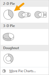
How to Make a Pie Chart in Excel: 10 Steps (with Pictures) Click the "Pie Chart" icon. This is a circular button in the "Charts" group of options, which is below and to the right of the Insert tab. You'll see several options appear in a drop-down menu: 2-D Pie - Create a simple pie chart that displays color-coded sections of your data. 3-D Pie - Uses a three-dimensional pie chart that displays color ...

33 How To Label A Pie Chart In Excel - Labels 2021

How to create a Pie chart in Excel - ablebits.com How to show percentages on a pie chart in Excel. When the source data plotted in your pie chart is percentages, % will appear on the data labels automatically as soon as you turn on the Data Labels option under Chart Elements, or select the Value option on the Format Data Labels pane, as demonstrated in the pie chart example above.. If your source data are numbers, then you can configure the ...

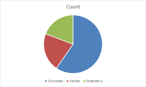
Pie Chart: Survey results favorite ice cream flavor | Exceljet

Office: Display Data Labels in a Pie Chart 2. If you have not inserted a chart yet, go to the Insert tab on the ribbon, and click the Chart option. 3. In the Chart window, choose the Pie chart option from the list on the left. Next, choose the type of pie chart you want on the right side. 4. Once the chart is inserted into the document, you will notice that there are no data labels.

33 How To Label A Pie Chart In Excel - Labels 2021

4 Ways To Add Data To An Excel Chart I said 4 ways so let's start with the first. 1. Copy Your Data & Click On Your Chart. So, let's add in some more data- another line in Row 10. Just copy the row data. Click on the outside of your chart. Hit Paste. Your chart will update. Easy as that.

Pie Chart: Survey results favorite ice cream flavor | Exceljet

How to display leader lines in pie chart in Excel? To display leader lines in pie chart, you just need to check an option then drag the labels out. 1. Click at the chart, and right click to select Format Data Labels from context menu. 2. In the popping Format Data Labels dialog/pane, check Show Leader Lines in the Label Options section. See screenshot: 3. Close the dialog, now you can see some leader lines appear. If you want to show all leader lines, just drag the labels out of the pie one by one.

Charts & Dashboards Archives - Page 2 of 5 - Excel Campus

How-to Add Label Leader Lines to an Excel Pie Chart - YouTube Step-by-Step Tutorial: how-to create label leader lines that connect pie labels that are outsi...

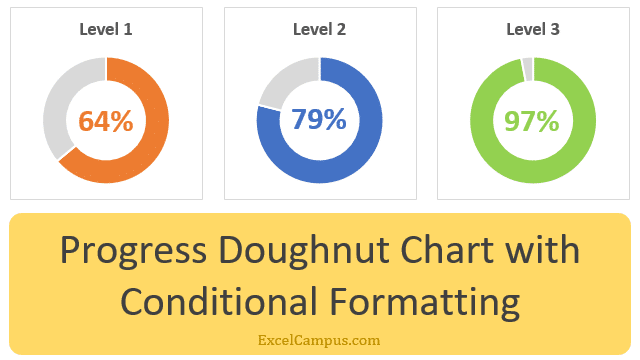
Excel Gauge Chart Template - Free Download - How to Create

How to Insert Axis Labels In An Excel Chart | Excelchat We will go to Chart Design and select Add Chart Element Figure 6 - Insert axis labels in Excel In the drop-down menu, we will click on Axis Titles, and subsequently, select Primary vertical Figure 7 - Edit vertical axis labels in Excel Now, we can enter the name we want for the primary vertical axis label.

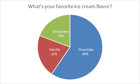
Pie Chart: Survey results favorite ice cream flavor | Exceljet

How to Create a Pie Chart in Microsoft Excel Create the Basic Pie Chart. You can create a pie chart based on your data in two different ways, both begin with selecting the cells. Be sure to only select cells that should be converted into the chart. Method 1. Select the cells, right-click on the chosen group, and pick Quick Analysis from the context menu. Under Charts

Share :